From the inbox here at SSEC, we received this request:

“As a user of GOES and Himawari data (through EUMETCast) I would like to use SIFT software. I have experimented a little and watched a couple of videos on the SIFT blog. But the latter offers a very limited range of material and assumes one has learnt the basics. Do you have a simple manual that an absolute beginner can use in order to get started with SIFT?”

The goal of this Blog Entry is to achieve this task. So:

1. SIFT was designed to allow users to interrogate Himawari-8 imagery (that was later expanded to GOES-R once GOES-16 — and then GOES-17 — was launched). Thus, it has animating capabilities, pan and zoom abilities, the ability to interrogate imagery, to compare bands, and to create channel differences and Red-Green-Blue composite imagery, because these are important aspects of investigating geostationary imagery.
2. SIFT is designed to be self-contained; that is, when you download it, all dependencies are included. Simply unzip and untar the install file (in unix world), or run the installer in Windows or Apple OS. You are then left with an executable link to start up.
3. When you start up SIFT, one window opens up. This includes links to load up data — a File/Open (or ctrl-o) that will open up a familiar-looking dialog box in which you navigate to GOES-R netCDF files (or either Radiance or Cloud/Moisture Imagery). Alternatively, you can point to Himawari files that have been processed with axi-tools to create netCDF files. Note: File I/O is changing after v 1.0.6; Himawari data will be directly importable, and ctrl-o will be replaced with a File Open Wizard (you’ll still be able to find this under the ‘File’ tab in the upper left portion of the SIFT window!)

Once the data are loaded, what can you do?

1. You can compare to bands/channels.
   • If you load up 16 bands at one time, for example, you can cycle through all bands (Use the up/down arrows to do this ; the right/left arrows will cycle through times if multiple times are loaded).
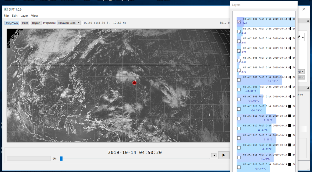
   • You can Probe all bands at once: Position the cursor at a location, and left-click. This will probe all data at that point, and values will show up in the Layers Window (as well as in the SIFT window, above the imagery, where the lat/lon will also be shown). See the figure below.
   • You can toggle between two images. For example, if you load up all 16 bands from GOES-16, but want to toggle only between Band 2 (the red visible at 0.64 micrometers) and Band 5 (the snow/ice/glaciation band at 1.61 micrometers) to highlight differences over frozen water and between land/water. Note that the Boundaries have been turned off (using the ‘B’ key) and that animation order has been specfied (using the ‘O’ key) and then clicking/unclicking the visibility of Band 3 — the 0.64)